def LinearFunc(x, weight, bias):
    """
    Linear function: y = weight * x + bias
    """
    return weight * x + bias

import math
# Generate some sample data
x = [i for i in range(10)]
y = [math.sin(i) for i in x]

def MSE(x, y, weight, bias):
    """
    Calculate the mean squared error (MSE) for a linear model.
    """
return sum((y[i] - LinearFunc(x[i], weight, bias)) ** 2 for i in range(len(y))) / len(y)Gradient descent: How do neural networks learn?
We have seen how you can prepare some data with features X and labels y. Then we can define the architecture/structure of a multi-layer perceptron (MLP) and randomly initialise a collection of weights w and biases b for the different neurons and layers of our MLP. We can then feed our training data through our MLP to get predictions of our class labels.
\(X_{i} \to MLP(w, b) \to Prediction_{i}\)
We have also seen that we can measure our mean squared error by adding up the squared difference between each prediction and the corresponding observation (i.e. the correct answer) and then dividing by the number of predictions. This value will be 0 if our predictions are all correct and will get larger as a larger proportion of our guesses are wrong.
\(Predictions, Observations \to Error\)
Tuning our weights and biases
We saw that randomly initialising the weights and biases was unlikely to lead to good predictions which means our error will start off quite high. We want to tune our weights and biases in a way that reduces that error.
The error is a function of our predictions and our observations. Our predictions are a function of our weights and biases. These statements together imply that our error is implicitly a function of our weights and biases. In other words:
Changing your weights and biases in your neural network will change your error.
For fixed data and network structure, we can try to understand how we can change our weights and biases to reduce our error.
Gradient Descent in 1D
Below you can pick different weights and biases for your linear model and see how they affect the MSE value
import matplotlib.pyplot as plt

weight = 1
bias = 0
Linear = [LinearFunc(i, weight, bias) for i in x]

plt.figure(figsize=(10, 6))
plt.plot(x, y, marker='o', label='Sine Function', color='blue')
plt.plot(x, Linear, label=f'y = {weight}x+{bias}', color='red', linestyle='--')
plt.legend()
plt.title(f'Sine Function vs. Linear Model; y = {weight}x + {bias}; MSE = {MSE(x, y, weight, bias):.2f}')
plt.xlabel('x')
plt.ylabel('y')
plt.grid()
plt.show()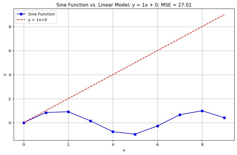
Now if we fix the bias but vary the weight we can see how that affects the MSE
# Fix the bias but vary the weight
bias = 2

ErrorDict = {}
for weight in range(-20, 20, 2):
    mse = MSE(x, y, weight, bias)
    ErrorDict[weight] = mse

# Plot the error curve
import matplotlib.pyplot as plt

plt.figure(figsize=(10, 6))
plt.plot(ErrorDict.keys(), ErrorDict.values(), marker='o')
plt.title('Mean Squared Error (MSE) vs. Weight (w1)')
plt.xlabel('Weight (w1)')
plt.ylabel('MSE')
plt.grid()
plt.show()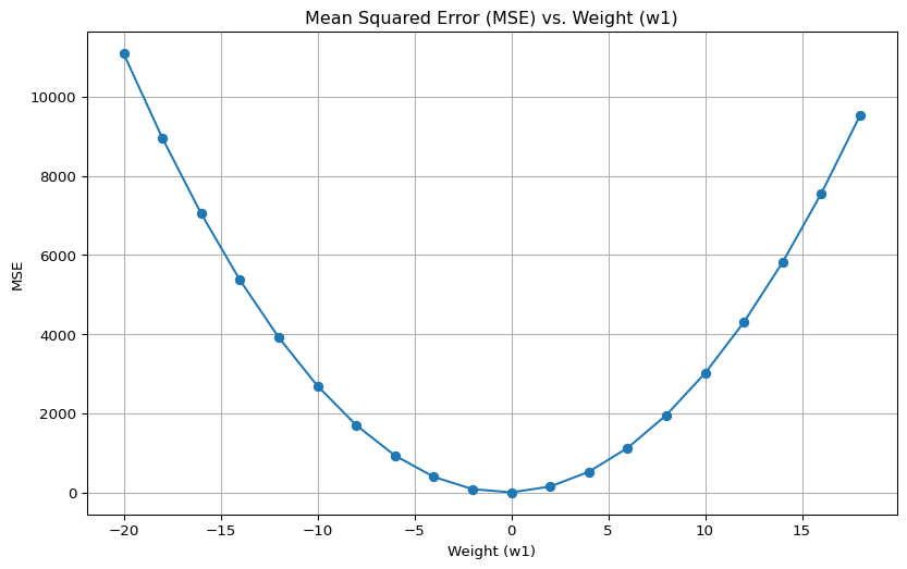
We can see for different weight values, there is a different error value. Accurate prediction is as simple as minimising the error with respect to the weights and biases.
In a calculus class you might have taken the derivative of a function \(\frac{dError}{dWeight}\), which represents the slope/gradient of the error function with respect to the weight at a given position. If you’re unfamiliar or rusty with calculus, you might want a refresher with something like YouTuber 3Blue1Brown’s Essence of Calculus Course.
Whilst you could in theory solve for when the derivative/slope is zero, to find an explicit answer in situations where there are a large number of weights and biases is often intractably difficult.
Instead, we understand that if the derivative is positive when the slope is upwards and negative when the slope is downwards, we can just head in the opposite direction of the derivative.
def DerivativeMSE(x, y, weight, bias):
    """
    Calculate the derivative of MSE with respect to weight.
    """
    return -2 * sum((y[i] - LinearFunc(x[i], weight, bias)) * x[i] for i in range(len(y))) / len(y)

# Create subplots
fig, axes = plt.subplots(1, 2)
fig.set_size_inches(12, 6)

# Plot MSE
axes[0].plot(ErrorDict.keys(), ErrorDict.values(), marker='o')
axes[0].set_title('MSE vs. Weight (w1)')
axes[0].set_xlabel('Weight (w1)')
axes[0].set_ylabel('MSE')
axes[0].grid(True)

# Plot Derivative of MSE
axes[1].plot(ErrorDict.keys(), [DerivativeMSE(x, y, weight, bias) for weight in ErrorDict.keys()], marker='o')
axes[1].set_title('Derivative of MSE vs. Weight (w1)')
axes[1].set_xlabel('Weight (w1)')
axes[1].set_ylabel('d(MSE)/dw1')
axes[1].grid(True)

plt.tight_layout()
plt.show()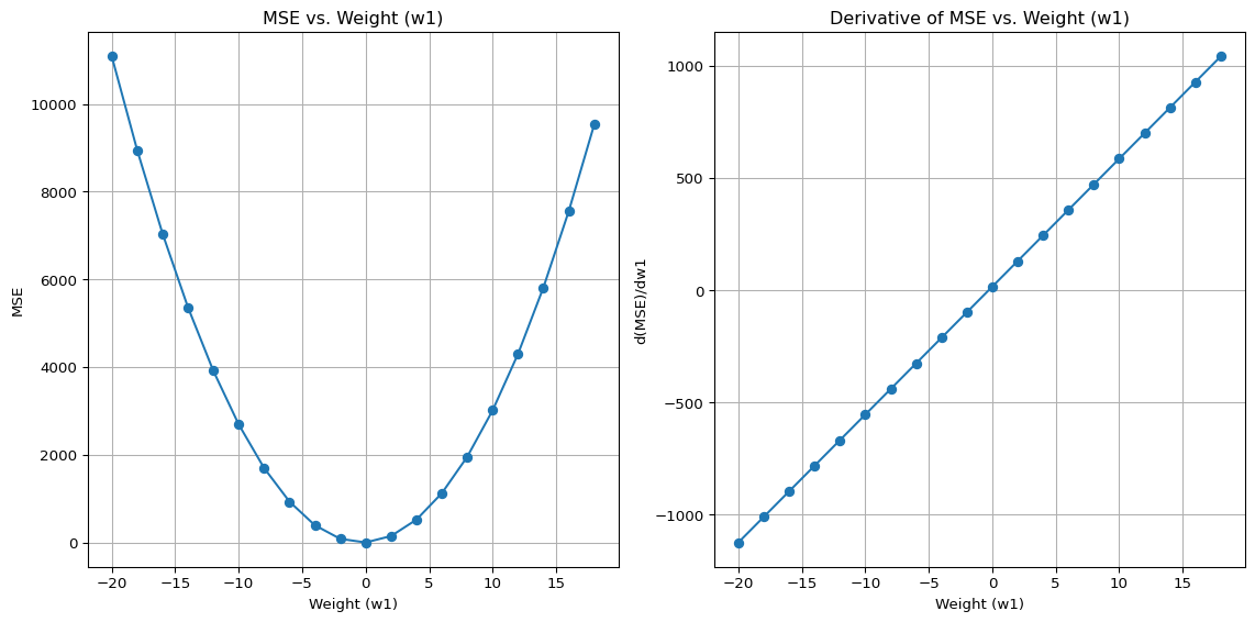
Consider the above left plot and choose a position on the x-axis and look at its corresponding MSE value. You can intuitively see which way is “downhill”.
On the above right plot you should be able to read off the derivative at the same x-axis value. If the left plot shows you’re facing uphill, the derivative should be positive on the right plot. If you’re facing downhill the derivative should be negative. The larger the value of the derivative, the steeper the slope.
Imagine you’re hiking in a misty mountain range and trying to get back to base camp at the bottom of the range, but you can’t see in front of you. All you can feel is the slope underneath your feet. What you might want to do is to feel the slope underneath you (i.e. the gradient of the ground) and take a step in the direction of that slope. Once you take a step, you stop, feel the ground underneath you again and decide on a new direction and step size.
If the slope is very big, you might take a larger step, assuming it will get you downhill faster. If the slope is very small you might take a smaller step so you don’t overshoot and start going uphill again. This is how gradient descent works!
In practise we take a step size proportional to the derivative/slope. We call the constant of proportionality the learning rate. If the learning rate is too large we might step over a minimum. If the rate is too small then we might take too long to find the minimum!
Gradient Descent in Higher Dimensions
In practise, we want to update all the weights and biases of our neural network at once. This means we want to use a generalisation of the derivative called the gradient function. Given a function \(f\) of \(n\) variables: \(w_{1}, w_{2}, \ldots, w_{n}\) we can define the gradient function of \(f\) as:
\(\nabla f (w_{1}, \ldots, w_{n}) = \begin{bmatrix} \frac{\partial f}{\partial w_{1}} \\ \frac{\partial f}{\partial w_{2}} \\ \vdots \\ \frac{\partial f}{\partial w_{n}} \end{bmatrix}\)
where \(\frac{\partial f}{\partial w_{1}}\) is the partial derivative of the function \(f\) with respect to \(w_{1}\). What this means is that each component of this vector tells you how steep the function \(f\) is with respect to each of its variables.
This just now means, if we think of our misty mountain range analogy from earlier, instead of only having to figure out if we need to walk north/south and east/west, we have a lot more directions to consider in gradient descent! The principle remains the same, even if visualising the geometry gets a little hazy.
You can play around with this web app to see how the loss surface “looks” with respect to a function and see how gradient descent moves you downhill towards minimal loss
https://neuralpatterns.io/hill_climber.html
Other optimisers
In practise, modern optimisers can perform better than standard gradient descent which often has problems getting “stuck” in areas that are minima but not the global minimum (imagine walking down hill until you get into a valley, or onto a little plateau which is not the bottom of the misty mountain range).
The general principles of these optimisers rely on gradient descent as a base line, but they are modified somewhat to get around this problem of getting stuck in local minima and to reduce the computational load of calculating gradients. You could think of the difference between standard gradient descent and stochastic gradient descent as that between a scout guide carefully working out the precise way to step every single time versus a bumbling hiker who is hastily making decisions about which way to walk every step. Their decisions are quicker to make and less effected by small irregularities of the mountain (and in practise, at least for neural networks, tend to perform better!)
Some of these methods include “Stochastic Gradient Descent” (SGD) and “Momentum Gradient Descent” (MGD) more info on these can be found here: