Data pipeline

This section builds a data pipeline which includes data loading, preprocessing, and batching with DataLoader. We will use the iris dataset from scikit-learn.

Step 1: Load and explore the Iris dataset

The Iris dataset is a classic dataset in machine learning practice containing measurements of sepals and petals from three species of iris flowers.

import pandas as pd
from sklearn.datasets import load_iris

# load the dataset
iris = load_iris()

# extract features and target classes
X = iris.data
y = iris.target
feature_names = iris.feature_names
target_names = iris.target_names

# Convert to DataFrame for easier manipulation
iris_df = pd.DataFrame(X, columns=feature_names)
iris_df['species'] = pd.Categorical.from_codes(y, target_names)

# Print the first few rows of the dataset to check its structure
print(iris_df.head())

# print to check the overall structure of our dataset
# and also to find how many classes we have
print(f"Dataset dimensions: {X.shape}")
print(f"Target classes: {target_names}")
print(f"Feature names: {feature_names}")

   sepal length (cm)  sepal width (cm)  petal length (cm)  petal width (cm)  \
0                5.1               3.5                1.4               0.2   
1                4.9               3.0                1.4               0.2   
2                4.7               3.2                1.3               0.2   
3                4.6               3.1                1.5               0.2   
4                5.0               3.6                1.4               0.2   

  species  
0  setosa  
1  setosa  
2  setosa  
3  setosa  
4  setosa  
Dataset dimensions: (150, 4)
Target classes: ['setosa' 'versicolor' 'virginica']
Feature names: ['sepal length (cm)', 'sepal width (cm)', 'petal length (cm)', 'petal width (cm)']

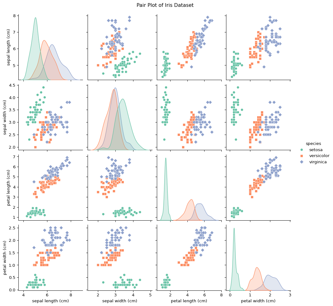
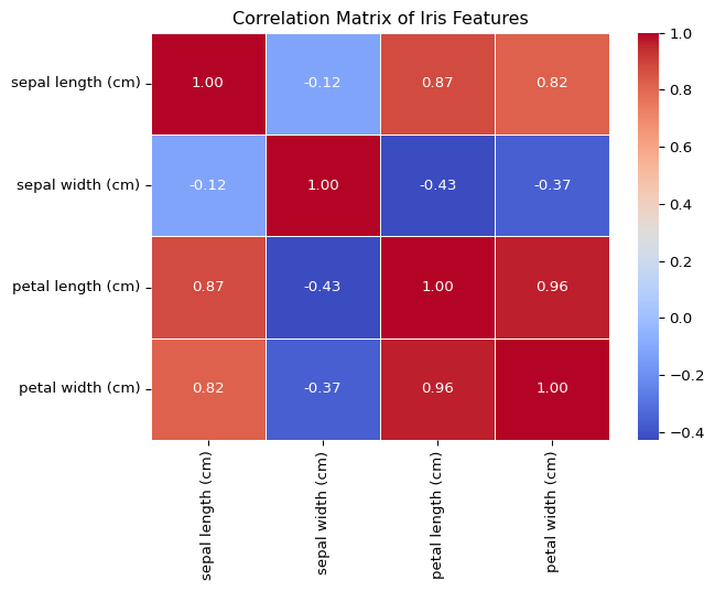
We have known that we have 150 samples and 4 features in our dataset, now let us visualize the relationships between these features using a pair plot. Additionally, we can also check the correlation matrix of the features to see how strongly the features are correlated with one another.

import matplotlib.pyplot as plt
import seaborn as sns

# Pair plot to visualize relationships between features
sns.pairplot(iris_df, hue='species', markers=["o", "s", "D"], palette="Set2")
plt.suptitle('Pair Plot of Iris Dataset', y=1.02) # Adjust title position
plt.show()

# check the correlation matrix of the features
corr_matrix = iris_df[feature_names].corr()
sns.heatmap(corr_matrix, annot=True, cmap="coolwarm", fmt=".2f", linewidths=0.5)
plt.title("Correlation Matrix of Iris Features")
plt.show()

Step 2: Split data into training and testing sets

We now divide our data into training and testing datasets in 80:20 ratio. This means, we will be using 80% of our data for training and 20% for evaluating the model’s performance.data

from sklearn.model_selection import train_test_split

# split data into training and testing sets with a seed for reproducibility
# X_train here contains training set for feature data
# y_train here contains target labels for training set, or what we want to predict, or the ground truth

X_train, X_test, y_train, y_test = train_test_split(X, y, test_size=0.2, random_state=42)

Step 3: Standarise or scale the feature data

Networks generally work better when the numbers are all the same order of magnitude. We want the network to learn how numbers vary, not their relative sizes to begin with.

from sklearn.preprocessing import StandardScaler

# standardise the feature data
scaler = StandardScaler()

# learn the parameter from training data and fit a transformer to it
# fit() - computes mean and std deviation to scale
# transform() - used to scale using mean and std deviation calculated using fit()
# fit_transform() - combination of both fit() and transform()
X_train = scaler.fit_transform(X_train)

# no fit() as we want to avoid data leakage
X_test = scaler.transform(X_test)

Now let us convert feature matrices to FloatTensor (tensor type for numerical data) and LongTensor (tensor type for “long” which is just a type of integer labels).

import torch
from torch.utils.data import DataLoader, TensorDataset

X_train_tensor = torch.FloatTensor(X_train)
y_train_tensor = torch.LongTensor(y_train)


X_test_tensor = torch.FloatTensor(X_test)
y_test_tensor = torch.LongTensor(y_test)

Step 4: Create tensor dataset and data loader for batch training

Whilst it is possible to use plain tensors for your training set, it can be advantageous to make use of PyTorch’s existing mechanisms for loading in data. This is particuarly relevant when we want to handle large amounts of data in effecient ways with multiple GPUs (e.g. using some kind of server or high performance computer). Below initialise a TensorDataset class for defining and accessing our data in an efficient way (we’ll talk about what a class is in the next section). The DataLoader class wraps the Dataset class and handles batching, shuffling, and utilise Python’s multiprocessing to speed up data retrieval.

# Combine features and labels into a single dataset
batch_size = 30
train_dataset = TensorDataset(X_train_tensor, y_train_tensor)
train_loader = DataLoader(dataset=train_dataset, batch_size=batch_size, shuffle=True)

test_dataset = TensorDataset(X_test_tensor, y_test_tensor)
test_loader = DataLoader(test_dataset, batch_size=batch_size, shuffle=False)

# Print batch information
print(f"Number of training batches: {len(train_loader)}")
print(f"Number of test batches: {len(test_loader)}")

Number of training batches: 4
Number of test batches: 1

Finally, our dataset is ready for model definition, training, and evaluation.

Next section will explain the model that we will utilise.