Understanding HPC resources

Before asking for time on an HPC system, you need to know how much you will need. Ask for too little and your jobs will be killed half way through; ask for too much and you will wait longer in the queue and waste a shared resource. This second part of the course shows you how to estimate the resources your project needs, starting from small, representative tests.

Intended learning outcomes

By the end of this part, you will:

• Understand the key HPC resource concepts: wall-clock time, CPU time and core-hours
• Know how to run representative benchmarks of your code
• Be able to use simple command-line tools to measure time and memory
• Be able to convert benchmark timings into a realistic resource request

Prerequisites

• Basic familiarity with the command line and the job scheduler (see the previous part)
• A computational task you want to benchmark

Key definitions

HPC allocations are usually measured in core-hours:

\[ \text{core-hours} \approx \text{wall-clock time (hours)} \times \text{number of CPU cores} \]

Term	Meaning
Wall-clock time	Elapsed time, as measured by a stopwatch
CPU time	Time the processors were actively working for you (excludes waiting for I/O)
Task	One independent run of your code (one simulation, one dataset, …)
Job	What you submit to the scheduler; it may contain many tasks

Example

A program that runs for 2 hours using 8 cores uses 2 × 8 = 16 core-hours.

CPU time versus wall time

The relationship between CPU time and wall-clock time tells you a lot about how your program behaves:

• Single core: CPU time ≈ wall time
• Multiple cores: CPU time ≈ wall time × number of cores in use
• I/O heavy (lots of reading and writing files, waiting for the network): wall time > CPU time

The Linux tool /usr/bin/time -v reports all of these. An example of its output:

Elapsed (wall clock) time (h:mm:ss or m:ss): 0:02:15
User time (seconds): 120.45
System time (seconds): 12.33
Maximum resident set size (kbytes): 2048000

Here the wall-clock time is 2 min 15 s (135 s) and the CPU time is the user plus system time (132.8 s), so the program was busy almost all the time on a single core. The maximum resident set size is the peak memory used: about 2 GB.

Tip

Understanding this relationship helps you optimise your resource requests: if the CPU time is much lower than the wall time multiplied by the cores you asked for, you are reserving cores that are sitting idle.

Why measure rather than guess?

Common mistakes

• Ignoring that HPC cores may be faster (or slower!) than your laptop
• “My laptop takes 1 hour, so I need 100 hours for 100 runs”: this ignores that the runs can be done at the same time
• Missing parallelisation opportunities
• Forgetting that there is some overhead in scheduling and starting jobs

Best practice

• Benchmark on the target system
• Use representative data
• Measure actual resource usage
• Account for variability between runs

Scaling laws

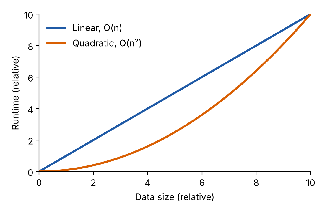
How does runtime grow with the amount of data?

The way the runtime grows when the problem gets bigger decides how you can extrapolate from a small test to the full problem.

Linear and quadratic growth of the runtime

Pattern	Behaviour	Typical example
Linear, O(n)	2 × data → 2 × time	Processing each file or record independently. Safe to extrapolate
Quadratic, O(n²)	2 × data → 4 × time	All-pairs comparisons, e.g. distance between every pair of points

Testing your scaling

Run your program with increasing fractions of your data and compare the times:

./my_program --data 2percent_sample.csv   # measure time
./my_program --data 4percent_sample.csv   # should take ~2x longer if linear
./my_program --data 8percent_sample.csv   # should take ~4x longer if linear

Warning

If the 8% sample takes 10× longer than the 2% sample (instead of 4×), you do not have linear scaling, and a straight-line extrapolation will underestimate the time needed for the full dataset.

Parallel scaling

When your code can use several cores, the time does not usually shrink in proportion to the number of cores. There are two ways of looking at this:

• Strong scaling: keep the problem size fixed and add cores. How much faster does it get?
• Weak scaling: increase the problem size in proportion to the number of cores. Does the runtime stay the same?

For strong scaling we define the speed-up and the parallel efficiency on \(N\) cores as

\[ S(N) = \frac{T(1)}{T(N)}, \qquad E(N) = \frac{S(N)}{N} = \frac{T(1)}{N \, T(N)} \]

where \(T(N)\) is the wall-clock time using \(N\) cores.

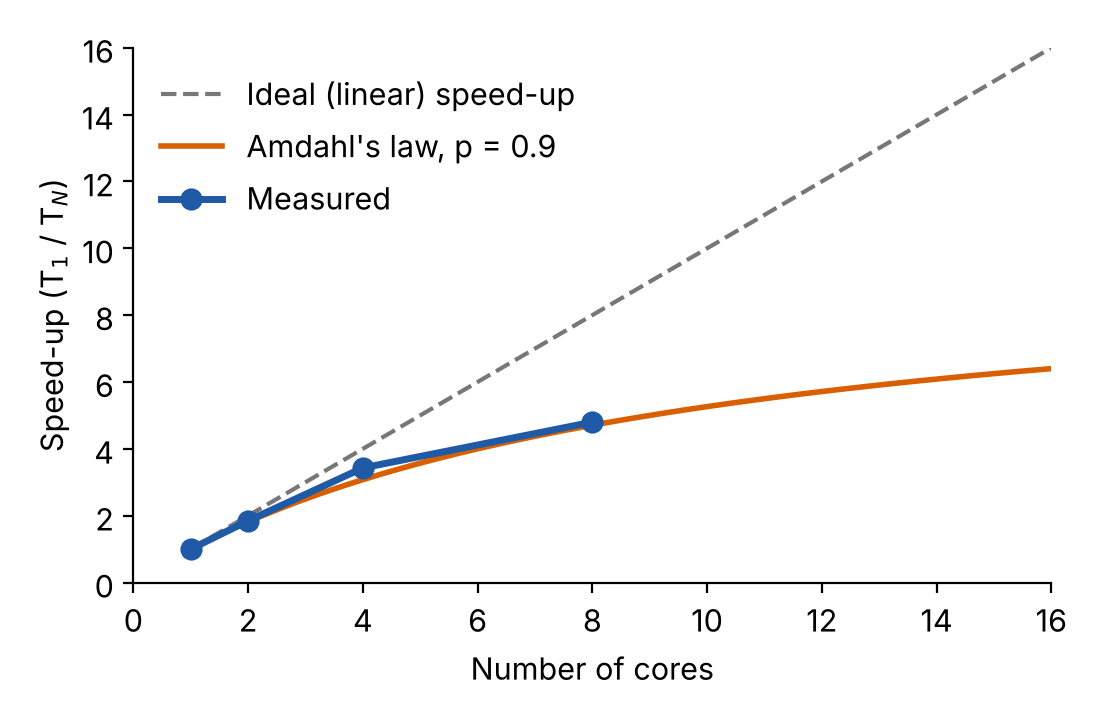
Amdahl’s law

Every program has some part that cannot run in parallel (reading the input, setting things up, …). If a fraction \(p\) of the work can be parallelised, the best possible speed-up on \(N\) cores is

\[ S(N) = \frac{1}{(1 - p) + p/N} \]

So even if 90% of your code is parallel (\(p = 0.9\)), you can never go more than 10× faster, however many cores you use.

Testing parallel scaling

#!/bin/bash
dataset="my_data.csv"

for cores in 1 2 4 8 16; do
    echo "Testing with $cores cores..."
    /usr/bin/time -f "cores=$cores wall=%E cpu=%U+%S" \
        my_parallel_program --input $dataset --threads $cores \
        2>> scaling_results.log
done

Example results

Cores	Wall time	Speed-up	Efficiency
1	120 s	1.0	100%
2	65 s	1.8	92%
4	35 s	3.4	86%
8	25 s	4.8	60%

Going from 4 to 8 cores only saves 10 seconds but doubles the core-hours used: 35 s × 4 = 140 core-seconds, against 25 s × 8 = 200 core-seconds. Using more cores is not always better value for your allocation!

Measured speed-up compared with ideal scaling and Amdahl’s law

Benchmarking your code