Fitting data

The process of extracting information from data using computers is called machine learning.

Machine learning a very large field and covers a whole host of techniques. In this course we will be discovering a few of them but let’s first start with the simplest form of machine learning, the linear fit or linear regression.

Input data

First we shall need some data. For this example we shall be pretending that we have measured these data from an experiment and we want to extract the underlying parameters of the system that generated them.

I have prepared a CSV file which you can read into pandas using read_csv:


import pandas as pd

data = pd.read_csv("https://bristol-training.github.io/applied-data-analysis-in-python/data/linear.csv")
data.head()

	x	y
0	3.745401	3.229269
1	9.507143	14.185654
2	7.319939	9.524231
3	5.986585	6.672066
4	1.560186	-3.358149

We can see here that the data has two columns, x and y. Traditionally, \(x\) is used for the things we can easily measure in the world and use as inputs, and \(y\) is used for the thing we want to predict. In our case, we want to work out what the value of \(y\) should be for any given \(x\).

In this case we have one single \(x\) column but in a more complicated data set we may have multiple \(x_1\), \(x_2\) etc. in which case the set together is sometimes given the upper-case letter \(X\). Each \(x_n\) column is called a feature. Features are usually things that you have measured as part of a experiment (e.g. height of a person, temperature of a room, size of a garden etc.).

Our \(y\) column is the thing that we are going to create a model to predict the value of. The \(y\) column of the input data is often called the label or the target.

Let’s check how many rows we have:

data.count()

x    50
y    50
dtype: int64

We have 50 rows here. In the input data, each row is often called a sample (though sometimes also called an instance, example or observation). For example, it could be the information about a single person from a census or the measurements at a particular time from a weather station.

Tidy data

Tidy data is data where:

Each variable is a column; each column is a variable.
Each observation is a row; each row is an observation.
Each value is a cell; each cell is a single value.

Let’s have a look at what the data looks like when plotted:

import seaborn as sns

sns.relplot(data=data, x="x", y="y")

We can clearly visually see here that there is a linear relationship between the \(x\) and \(y\) values but we need to be able to extract the exact parameters programmatically.

Linear regression

Setting up our model

For this and for the other machine learning techniques in this course, we will be using scikit-learn. It provides a whole host of tools for studying data. You may also want to investigate statsmodels which also provides a large number of tools for statistical exploration.

scikit-learn provides a number of models which you can use to study your data. Each model is a Python class which can be imported and used. The usual process for using a model is:

Import the model you want to use
Create an instance of that model and set any hyperparameters you want
Fit the model to the data, this computes the parameters of the model using machine learning
Predict new information using the model

As we saw by plotting the data, the relationship between \(x\) and \(y\) is linear. In scitkit-learn, linear regression is available as scikit-learn.linear_model.LinearRegression.

We import the model and create an instance of it. By default the LinearRegression model will fit the y-intercept, but since we don’t want to make that assumption we explicitly pass fit_intercept=True. fit_intercept is an example of a hyperparameter, which are variables or options in a model which you set up-front rather than letting them be learned from the data.

from sklearn.linear_model import LinearRegression

model = LinearRegression(fit_intercept=True)
model

LinearRegression()

In a Jupyter environment, please rerun this cell to show the HTML representation or trust the notebook.
On GitHub, the HTML representation is unable to render, please try loading this page with nbviewer.org.

When running a Jupyter Notebook, you will see this model summary box appear every time a cell evaluates to the model itself. Here, writing model causes this to happen explicitly but it will happen any time the last line in a cell has the return value of the model too.

Fitting the data

Once we have created our model, we can fit it to the data by calling the fit() method on it. This takes two arguments:

The input data as a two-dimensional structure of the size \((N_{samples}, N_{features})\).
The labels or targets of the data as a one-dimensional data structure of size \((N_{samples})\).

In our case we only have one feature, \(x\), and 50 data points so it should be in the shape \((50, 1)\). If we just request data["x"] then that will be a 1D array (actually a pandas Series) of shape \((50)\) so we must request the data with data[["x"]] (which returns it as a single-column, but still two-dimensional, DataFrame). For a more thorough explanation of this dimensionality difference, see this explanation.

If you’re using pandas to store your data (as we are) then just remember that the first argument should be a DataFrame and the second should be a Series.

X = data[["x"]]
y = data["y"]

model.fit(X, y)

LinearRegression()

It is when you call this function that scikit-learn will go away and perform the machine learning algorithm. In our case it takes a fraction of a second but more complex models could take hours to compute.

By the time that this function returns, the model object will have had it’s internal parameters set as best the algorithm can do in order to predict \(y\) from \(x\).

We see the summary box appear here too as the fit method returns the model that it was called on, allowing you to chain together methods if you want.

Making predictions using the model

Once we’ve performed the fit, we can use it to predict the value of new data points which weren’t part of the original data set.

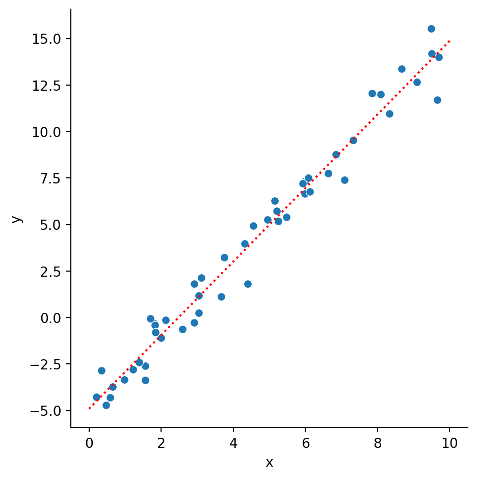
We can use this to plot the fit over the original data to compare the result. By getting the predicted \(y\) values for the minimum and maximum \(x\) values, we can plot a straight line between them to visualise the model.

The predict() function takes an array of the same shape as the original input data (\((N_{samples}, N_{features})\)) so we put our list of \(x\) values into a DataFrame before passing it to predict().

We then plot the original data in the same way as before and draw the prediction line in the same plot.

pred = pd.DataFrame({"x": [0, 10]})  # Make a new DataFrame containing the X values
pred["y"] = model.predict(pred)  # Make a prediction and add that data into the table
pred

	x	y
0	0	-4.903311
1	10	14.873255

import seaborn as sns
sns.relplot(data=data, x="x", y="y")
sns.lineplot(data=pred, x="x", y="y", c="red", linestyle=":")

As well as plotting the line in a graph, we can also extract the calculated values of the gradient and y-intercept. The gradient is available as a list of values, model.coef_, one for each dimension or feature. The intercept is available as model.intercept_:

print(" Model gradient: ", model.coef_[0])
print("Model intercept:", model.intercept_)

 Model gradient:  1.9776566003853107
Model intercept: -4.9033107255311155

The equation that we have extracted can therefore be represented as:

\[y = 1.97 x - 4.90\]

The original data was produced (with random wobble applied) from a straight line with gradient \(2\) and y-intercept of \(-5\). Our model has managed to predict values very close to the original.

Exercise

Run the above data reading and model fitting. Ensure that you get the same answer we got above.
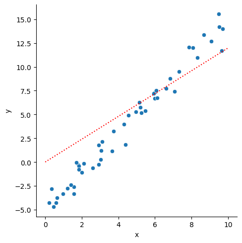
Try fitting without allowing the y-intercept to vary. How does it affect the prediction of the gradient?

Answer

import pandas as pd

data = pd.read_csv("https://bristol-training.github.io/applied-data-analysis-in-python/data/linear.csv")

from sklearn.linear_model import LinearRegression

model = LinearRegression(fit_intercept=False)
X = data[["x"]]
y = data["y"]
model.fit(X, y)

LinearRegression(fit_intercept=False)

pred = pd.DataFrame({"x": [0, 10]})
pred["y"] = model.predict(pred)

import seaborn as sns

sns.relplot(data=data, x="x", y="y")
sns.lineplot(data=pred, x="x", y="y", c="red", linestyle=":")

<Axes: xlabel='x', ylabel='y'>

print(" Model gradient: ", model.coef_[0])
print("Model intercept:", model.intercept_)

 Model gradient:  1.1985226874421444
Model intercept: 0.0